Geometric adstock explained: where a euro of outdoor actually lands

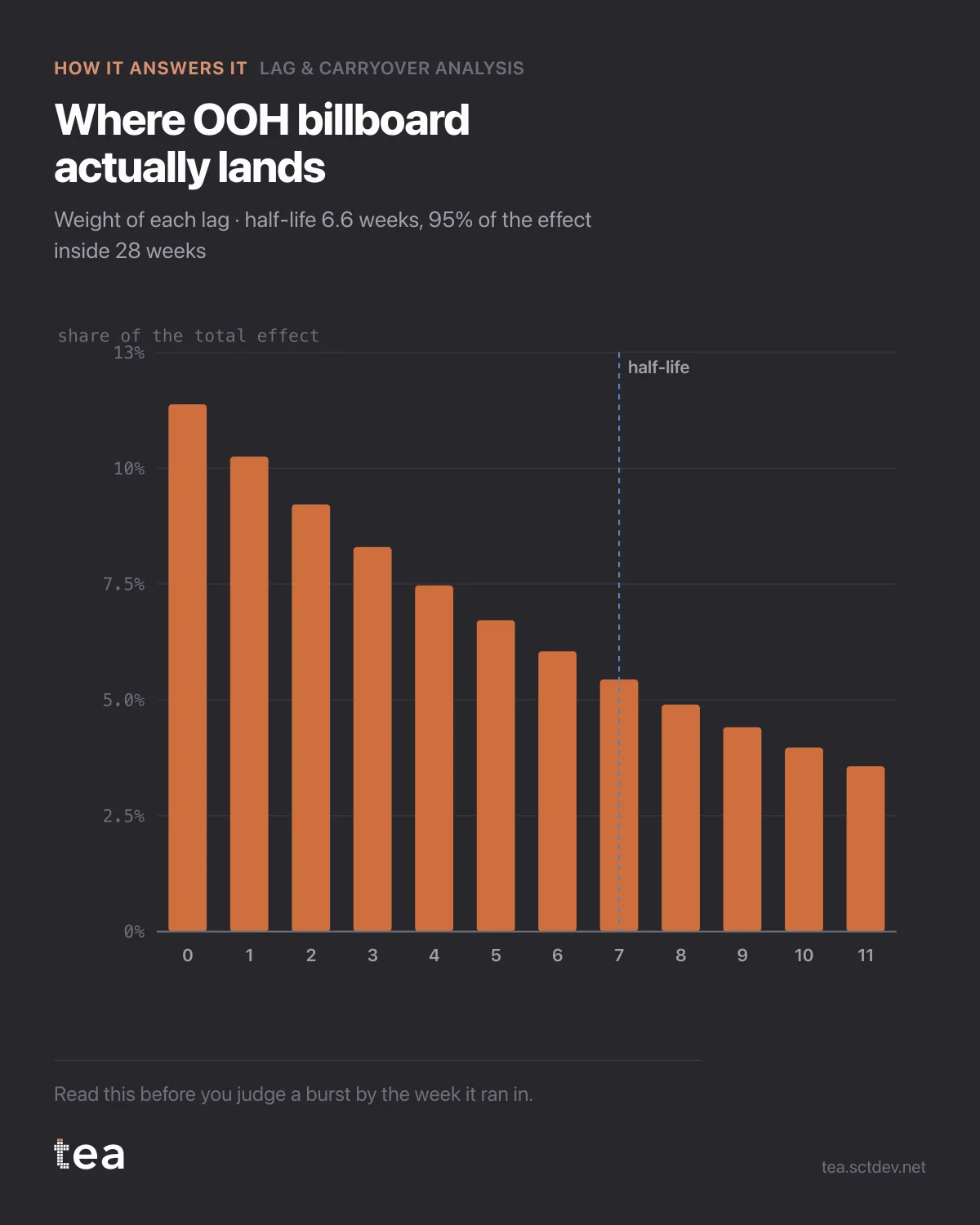
Where does a euro of outdoor actually land? Not in the week it ran, and this is the distribution.

Each bar is the share of the total effect that arrives at that lag. Week zero takes 13%. The rest is spread over the weeks after it, with a half-life of 6.6 weeks and 95% of the effect inside 28.

The shape is the point. It is not a spike with a bit of noise afterwards, and it is not a flat smear. It is a decay, and the rate of that decay is a property of the channel that you can estimate rather than assume.

How it is estimated, in plain terms. A geometric adstock transforms the spend series: each week carries a fraction of the week before, governed by one decay parameter. The model fits that parameter by trying a grid of candidates and keeping the one that explains the KPI best. Here it lands at 0.90, which is what produces a 6.6 week half-life.

Three cautions that come with it, and TEA prints all three.

The fit quality varies enormously by channel. Outdoor here reaches an R² of 0.53. Paid search, in the same file, reaches 0.07 and the regime is reported as uncertain rather than dressed up as a number. A decay estimated on a channel the KPI barely responds to is a decimal point with nothing behind it.

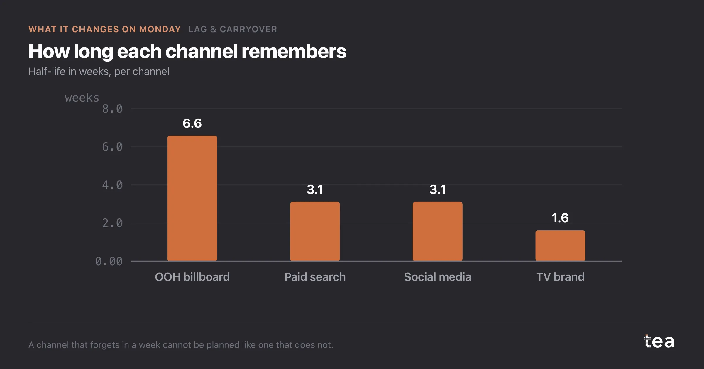
The decay and the effect size are estimated together, and they trade off. A model can explain the same history with a big immediate effect and fast decay, or a smaller effect that lasts. Which one it picks depends on how much variation the spend actually has. Flight patterns that never change give the model nothing to separate, which is why always-on channels are the hardest to read.

And a single channel fitted alone carries everything correlated with it. If outdoor runs when TV runs, its decay absorbs part of TV. The way out is to fit the drivers together, which is a different analysis and the honest next step.

Read this before you judge a burst by the week it ran in. Then read it again before you agree a reporting cadence.

If you only take one number from this chart, take the 95% window rather than the half-life. The half-life is the elegant statistic. The window, 28 weeks here, is the one that tells you when a flight has finished paying out, and that is the date a report should be written against.

It is also the number that makes finance comfortable. A channel with a six month tail is a channel whose budget cannot be judged inside a quarter, and saying so with a fitted curve is very different from saying so with an opinion.

The chart is the actual output of Lag & Carryover Analysis in TEA.