Why flat always-on spend makes carryover impossible to measure

Online home-insurance broker in Spain, always-on paid social at about €38k a week, asking what an August pause would cost.

A composite case, built from the kind of file we see most weeks. An online home-insurance broker in Spain, selling direct, with paid social as its largest channel. Spend had sat at about €38k a week for seventy weeks. Leads, meaning quote requests, ran at around 4,200 a week.

Finance wanted to pause social for August. The marketing lead wanted a number before agreeing, and the question came to us like this: "If we switch social off for four weeks, how fast do quotes drop, and how long does it take to get them back?"

That is a carryover question, and a good one. It is also one this file could not answer.

What the data looked like

Seventy weekly rows. Quote requests, paid social spend, paid search spend, a price index for the main product and a flag for the two weeks when the website was down.

The social column was the problem, and it was a problem because it was so well managed. The lowest week was €36.2k, the highest €39.9k. The coefficient of variation, the standard deviation divided by the mean, was 3%. No pauses, no bursts, no test weeks. A planner would call it disciplined. A model calls it silent.

Why adstock cannot be estimated here

Lag & Carryover works by asking how much of last week's spend is still visible in this week's result. In the outdoor case that question had an answer because there were bursts followed by quiet weeks, and the tail of each burst could be watched fading.

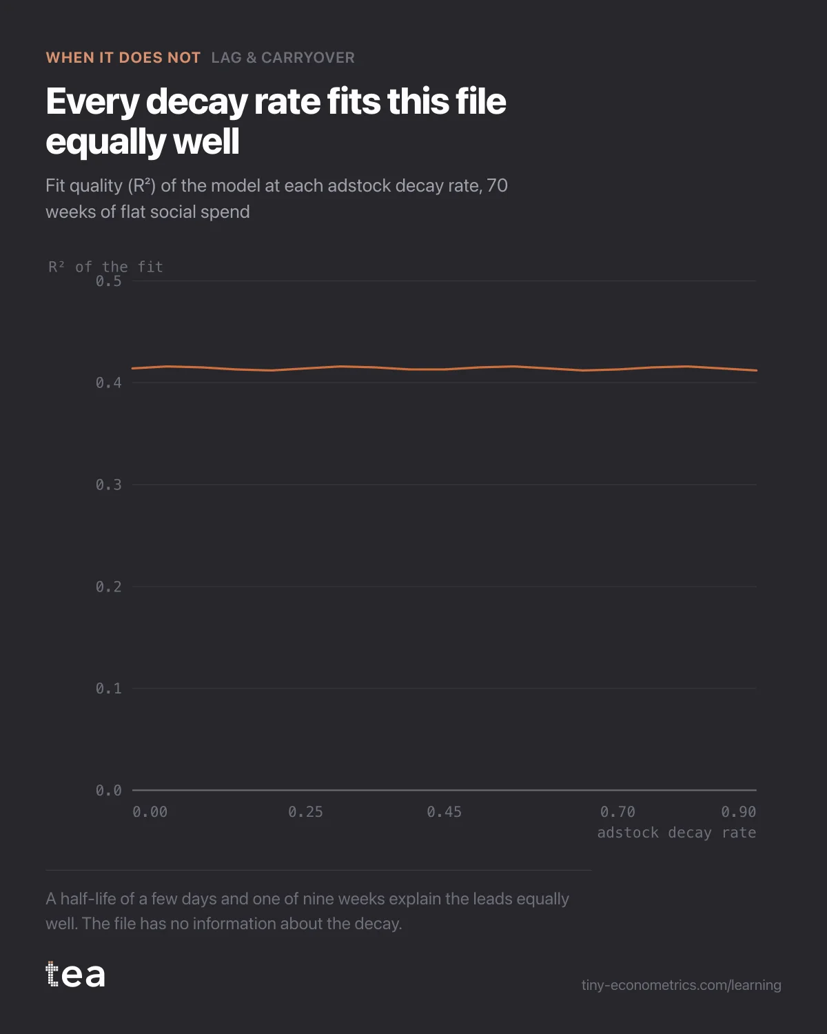
Here there is no tail to watch. When spend is the same every week, the adstocked spend is also the same every week, whatever the decay rate. A decay of 0.2 gives a flat line at about €47k of "effective" spend. A decay of 0.9 gives a flat line at about €380k. The two lines have the same shape, and the regression simply scales the coefficient to match. The data cannot tell them apart because, from the data's point of view, they are the same variable.

You can see it in the fit. Across every decay rate from 0 to 0.9, the R² of the model stayed between 0.41 and 0.42. tea returned a central decay of 0.48 with a 95% interval from 0.05 to 0.93. In half-lives, that is anything from a fifth of a week to 9.6 weeks. The report flagged the column as too thin to estimate a carryover, and that flag is the honest result.

There is a second, quieter problem. With spend that never moves, the effect of social itself is hard to separate from the baseline. The intercept and the social coefficient are both trying to explain the same constant level of leads, and the split between them is close to arbitrary.

What would have gone wrong if forced

Suppose someone took a benchmark half-life of three weeks off a slide and planned the pause on that. Two outcomes are plausible from this file, and they lead in opposite directions.

If the true half-life is short, quotes fall within days of the switch-off, the team panics, and the pause is reversed in week two at a cost. If it is long, quotes barely move in the first fortnight, the team concludes social was doing nothing, and the channel is cut for good in September, just as the tail runs out. August also carries its own seasonality for insurance quotes, which would be blamed on social or credited to it depending on the direction.

Either way, a decision gets made on a number the file never contained.

What to do instead

The fix is not a better model. It is a different file, and there are three ways to get one.

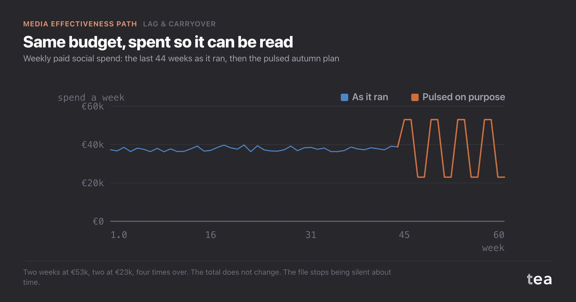
• Pulse on purpose. Keep the same total but alternate: two weeks at €53k, two at €23k, four times over sixteen weeks. Same budget, enough contrast for the decay to show itself.
• Run a geo holdout. Switch social off in three of Spain's larger provinces for six weeks, chosen to match the rest on past quote volume, and leave everything else alone. The comparison is the carryover, measured directly. The resulting file can later be read with Geo / Segment MMM.
• Make the August pause the experiment. If it is going to happen anyway, pause cleanly on a known date, change nothing else that month, and ideally pause only half the country.

The broker chose the pulsed plan for autumn and a regional pause for August. Neither costs extra money. Both cost a little comfort.

The lesson

A channel that never moves cannot tell you how long it remembers. Always-on spend is a sensible default for reach, but if you also want to measure it, some of the weeks have to be different on purpose.