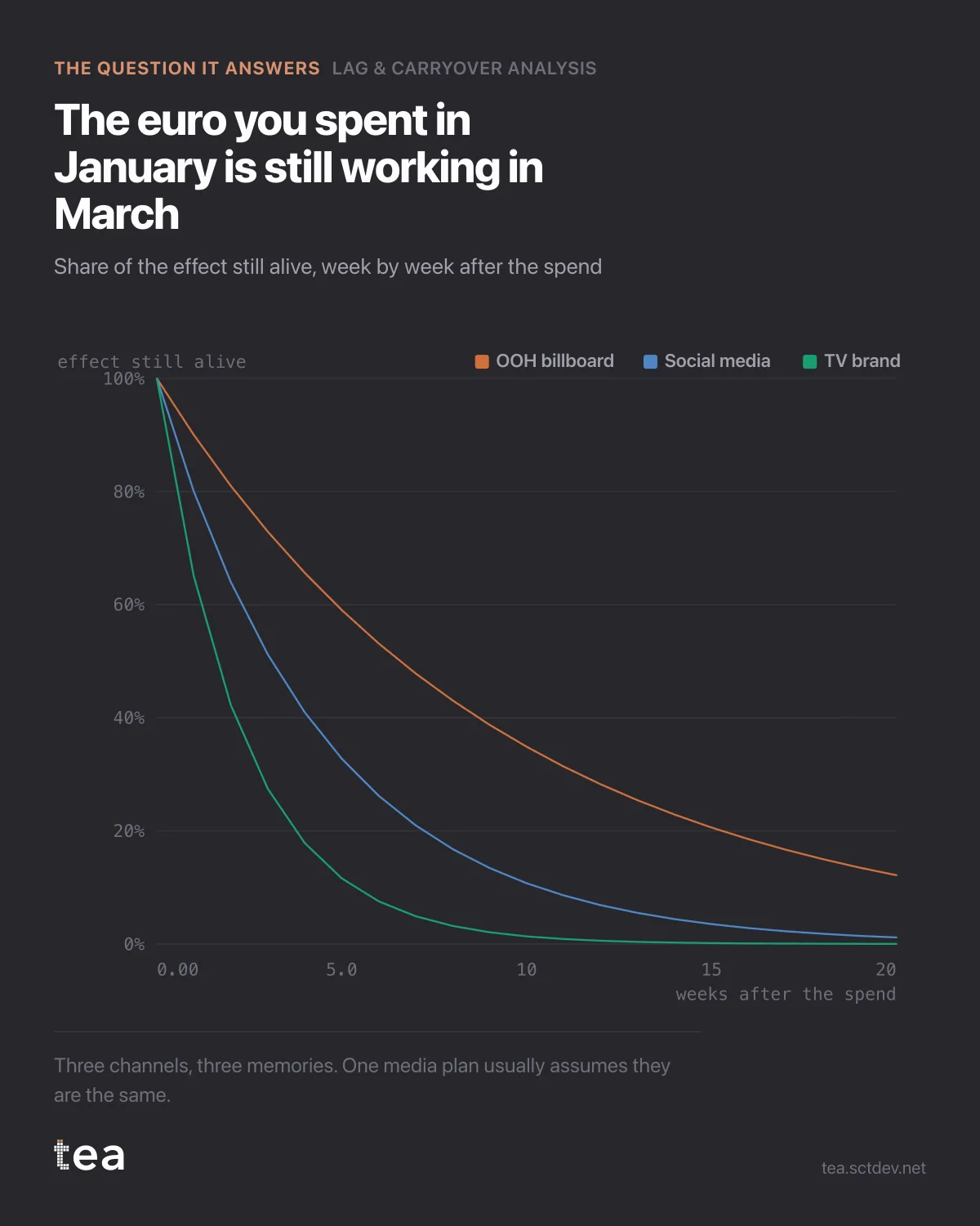
The euro you spent in January is still working in March. That is not a slogan, it is a measurable quantity, and this chart is what it looks like.
Three channels from two years of weekly data. Each curve is the share of a channel's effect still alive, week by week after the money left.
They do not decay at the same speed, and that is the finding.
OOH billboard has a half-life of 6.6 weeks. Half of what a burst will ever do has not happened yet a month and a half later, and 95% of it is still arriving inside 28 weeks.
Social media sits at 3.1 weeks. TV brand, in this file, at 1.6.
Now hold that against how media is usually judged. A flight runs in week 12. The report lands in week 14. Whatever the numbers say, they are reading a fraction of the result, and the fraction is different for every channel in the plan.
The consequences are not subtle.
A channel with long memory looks weak in a fortnightly report and strong in a quarterly one, so its budget depends on the reporting cadence rather than on its performance. Nobody decided that. It is just what happens when a decay of six weeks meets a review cycle of two.
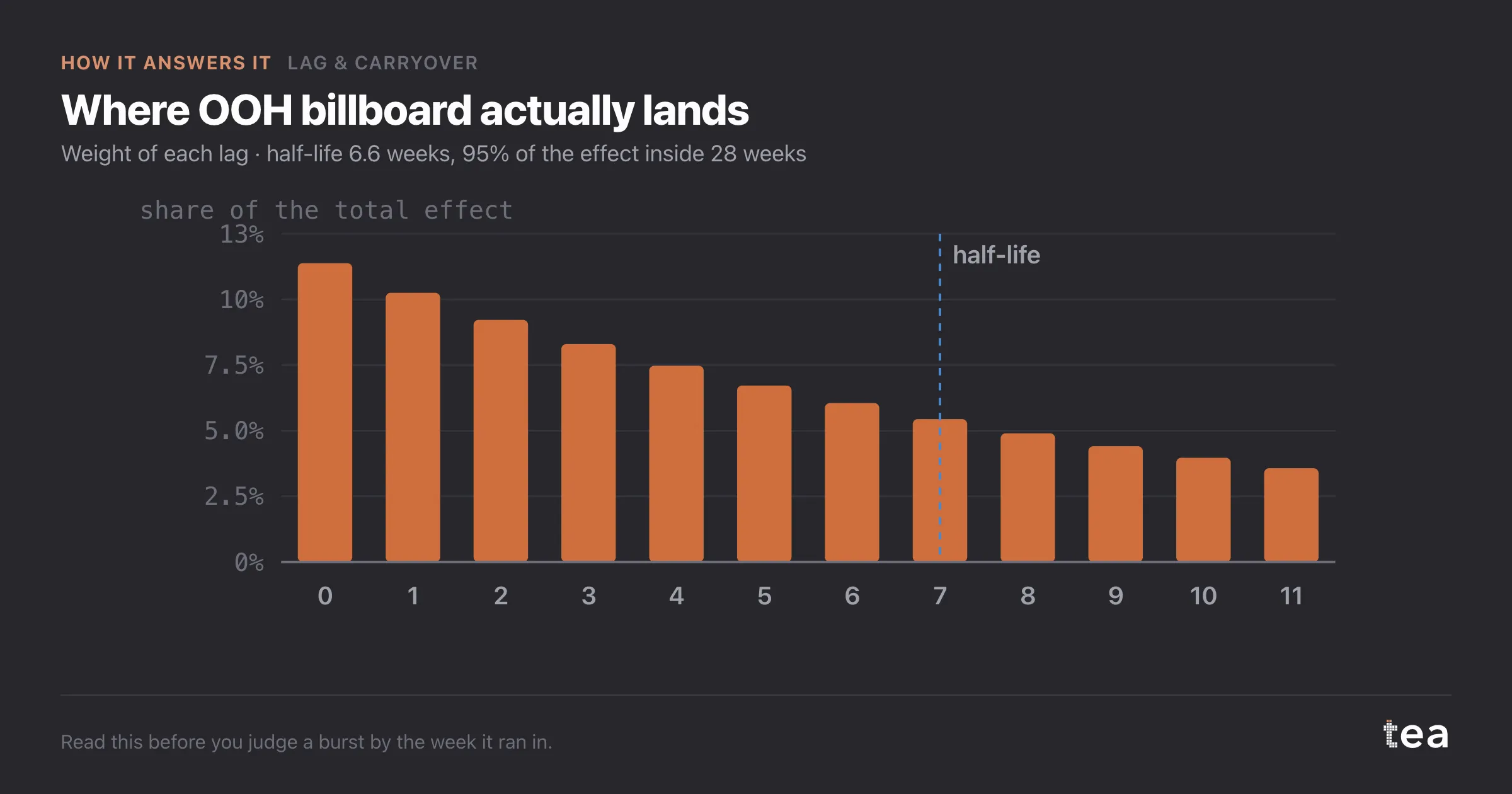
Turning a long channel on and off wastes the tail. Stopping a 6.6 week half-life channel to fund a burst somewhere else buys you the burst and pays for the silence twice, once in what stops arriving and once in the rebuild.
And comparing channels on last-click, or on any same-week measurement, is comparing how fast they report rather than how well they work. The fast channel wins every time, by construction.
The model here is a geometric adstock. One parameter, the decay rate, estimated on your own data rather than assumed from a benchmark table. The output is the half-life, the window that holds 95% of the effect, and a cumulative multiplier that tells you how much more the channel is worth over its life than in the week it ran.
Two years of weekly spend and one KPI column. That is the entire input.
A practical note on reading the curves. What matters is not the exact half-life to two decimals, it is the ranking and the order of magnitude. Six weeks against one and a half is a difference you can plan around. Six point six against six point two is a difference you should ignore, and the fit quality will usually tell you which of the two situations you are in.
The other thing this changes is how you argue for brand spend. The case for it is usually made with theory and a chart from a book. This is the same case made with your own series, in weeks, with your own channels in it, which is a considerably shorter meeting.
The chart is the actual output of Lag & Carryover Analysis in TEA, run on a sample file anyone can download.