ea

Analyses/Media Effectiveness Path/Lag & Carryover

How long a euro of media keeps working.

Lag & Carryover measures the memory of each channel: how much of a burst lands in the weeks it runs, and how much arrives after the posters come down. Before anyone asks how big an effect was, it finds out how long it lasts.

Answers How long does this channel keep working? Needs Weekly or daily KPI, spend per channel, spend that moves Hands back Decay rate, half-life, 95% window, per channel

A three-week burst, and the eight weeks it really worked

weekly spend and the sales it moved, €k
  • Spend
  • Sales moved by the burst
While it ran46%of the effect, weeks 1 to 3
The five weeks after43%invisible to a same-week report
Half-life2.1 weeksa decay of 0.72 a week

The outdoor and radio burst of a furniture retailer, from the first example below. A composite case: your file draws its own decay, channel by channel.

01

What it is for

Media does not work on the day it is bought. A radio spot is heard, remembered, talked about, and acted on later. Carryover is the share of the effect that arrives after the week the money was spent, and every channel carries a different amount of it.

Reading a burst on the right window

A channel with a two-week half-life judged on the weeks it ran loses half its result before the report is written. The window should follow the memory, not the calendar.

Planning flights and pauses

How long a pause can last before sales notice. How far apart two bursts can sit before the second one starts from zero. Both are half-life questions.

Feeding every model that follows

Saturation curves and the decomposition are fitted on spend as it works, spread over weeks, not as it was booked. Without the decay, slow channels look weak and fast ones look brilliant.

02

How to read it

One block per channel. A label that tells the story in two words, four numbers that defend it, and two charts. Read them in this order.

Outdoor + radio Balanced memory1
λ = 0.722 Half-life 2.13 95% window 94 R² 64%5

Decay curve

Impulse response

  1. The regime. Immediate and short, balanced, slow-build and long, or uncertain. It is the sentence you say in the meeting, and the one to check first: uncertain means the numbers beside it are not to be quoted.
  2. The decay rate, λ. The share of this week’s effect still alive next week. 0.72 means each week keeps 72% of the one before. tea tries every value from 0.05 to 0.95 and keeps the one that fits best, so read it with the fit beside it.
  3. The half-life. The same number on a clock: the periods it takes for half the remaining effect to arrive. It is in the unit of your file, weeks here, days on a daily file.
  4. The 95% window. How long until 95% of the effect has landed. This is the reading window for a report, and it is always much longer than the half-life: about four times, with a geometric decay.
  5. The fit, R². How much of the KPI the adstocked spend explains. Low is not wrong, but when R² barely moves across decay rates, the file is not telling one memory from another.

03

Where it sits in the analysis

Lag & Carryover opens the Media Effectiveness Path, the path that ends in a reallocation rather than in a report. It comes first for a plain reason: the size of an effect cannot be measured before its length is known, or the tail of every burst is counted as baseline.

What you carry into the next step is one number per channel, the decay rate. Every analysis below it uses that number without asking again.

It is also where a Time Series run sends you: a media effect that lands weeks later looks like autocorrelation to ARIMA, and is better measured directly.

Media Effectiveness Path

  1. Lag & Carryover this page

    Finds how long a burst keeps working, before anyone tries to measure how big it was.

    Carries forward: adstock rate per channel

  2. Saturation Curves

    Where each channel stops paying back, fitted as a curve rather than asserted as a rule of thumb.

  3. Contribution & Driver Decomposition

    What each channel actually contributed across the window, adstock and saturation included.

  4. Budget Optimization

    The same budget, moved. With the conservative scenario for when the plan meets reality.

  5. Geo / Segment MMM optional

    The same model per region or segment, if your file carries one. Where the average hides two different markets.

04

Where it usually misleads

The maths of adstock is simple and rarely the problem. The problems are in the file and in the reading, and none of them makes the software complain.

Spend that never moves

With the same spend every week, the adstocked series is a flat line whatever the decay, and the model cannot tell a half-life of one day from one of ten weeks. Any half-life fits as well as any other. Second example below.

A spend column that never changes is refused, and a channel whose fit explains under 15% of the KPI is labelled uncertain. Nearly flat spend can pass both: look at how much your spend moves before quoting the half-life, and pulse it if it barely does.

Channels that always run together

Outdoor and radio booked in the same weeks, at the same ratio, have one memory between them. Any split of it is invented. The honest result is a single decay for the pair, said on the first line.

Each channel is fitted on its own, so both of a pair get a decay even when they always ran together. If two columns move in step, add them into one column in your file and run them as one channel.

Half-life read as “how long it works”

A half-life of two weeks does not mean the effect is over in two weeks. Half of what remains is still to come, and 95% of it takes about nine. Reading the half-life as the window cuts the tail in two.

The 95% window sits beside the half-life on every channel.

Trend and season taken for memory

A burst in November is followed by Christmas. A burst in a growing year is followed by growth. Both look like a long tail. A decay estimated without the calendar credits the calendar to media.

Each channel is fitted without controls, so read a tail that ends at Christmas with suspicion. Run Trend and Seasonality first to see the calendar, and use Contribution Decomposition when the decay and the season have to share one model.

A benchmark half-life from a slide

“TV lasts three weeks” is an average over other brands, other creatives and other markets. Planned on, it can make a pause look free or ruinous, and the file never had a say.

No benchmark decay is ever filled in: λ is the value between 0.05 and 0.95 that fits your file best, and a channel whose fit explains under 15% of the KPI is labelled uncertain.

A clock too coarse for the channel

On monthly data, a search effect that fades in four days is invisible: it all lands in the month it was bought. A short half-life on a coarse file is a lower bound, not a finding.

The half-life is counted in the periods of your file, weeks on a weekly file, months on a monthly one. On monthly data, read a half-life under one period as a lower bound.

05

Two examples

One file where the analysis changed a decision, one where it could not answer. Both are useful results.

Helps

The outdoor burst judged on the wrong week

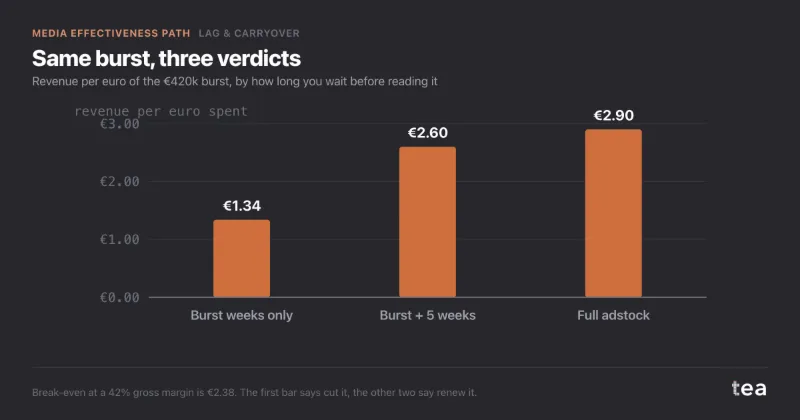
A furniture retailer with 38 stores in northern Italy ran three weeks of outdoor and radio, €420k. The internal report read sales during those weeks and found €1.34 back per euro, against €2.38 needed to break even at a 42% margin. The burst was about to be cut.

Four bursts over two years, with quiet weeks between them, gave the tail somewhere to show. The decay came out at 0.72, a half-life of 2.1 weeks. Summed over the whole tail, the burst returned €2.90 per euro. The autumn burst was renewed, and the reading window became “the weeks it ran plus five”.

Read the full case

Return per euro, by reading window

€ of sales per € spent

The same burst, three windows. Only the first one is below break-even.
Does not help

Seventy weeks of identical spend

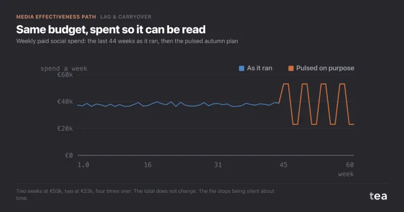
An online insurance broker in Spain wanted to know what an August pause of paid social would cost. Spend had sat at €38k a week for seventy weeks, with a 3% coefficient of variation. A planner would call it disciplined. A model calls it silent.

Every decay from 0 to 0.9 fitted equally well, R² between 0.41 and 0.42. The best fit was a coin toss: any half-life from a fifth of a week to 9.6 weeks explained the file as well as any other. The answer was not a number but a design: four alternating pulse weeks, or a geo test, before August.

Read the full case

Eleven decay curves, one fit

share of the effect still ahead, by week

Any of these curves explains the file as well as the others. The width of the fan is the result.

06

What the charts add to the numbers

A decay rate is one number, and one number invites one reading. Each chart turns it into a question a planner actually asks, and the comparison view turns four channels into a schedule.

Decay curve

how much is still ahead

Reads as: if we stop today, how much of what we bought has not arrived yet. The dashed line marks the half-life, so the clock and the curve are read together. It is the chart for a pause.

Impulse response

where one euro lands, week by week

Reads as: how a single euro spreads over the following weeks. The bars are the reading window drawn: wherever they are still visible, a report that has stopped counting is undervaluing the channel. It is the chart for a post-campaign review.

Comparison view

four channels on shared axes
  • Paid search · half-life 0.5
  • Paid social · half-life 0.9
  • Outdoor + radio · half-life 2.1
  • TV · half-life 3.5

Reads as: which channels are sprinters and which carry weight for weeks. Overlaid, the curves give the order of a flight: the long-memory channel opens, the short one closes, and the gap between two bursts of the same channel should not exceed its window. Check the regime of each channel before you plan on its curve: an uncertain one is drawn like the others.

tea, the product

Measure the memory of your own channels

A CSV with a date, a KPI and the spend per channel. The decay, the half-life, the window and the fit, in minutes, and a plain sentence when the relationship is too weak to plan on. Free while in beta, by invitation.

Request a place in the beta

tea, the product

Fifteen econometric analyses on your own CSV: Lag & Carryover, saturation curves, elasticities, budget allocation. The diagnostics shown, and a plain sentence when the file cannot answer.

Free while in beta, by invitation.

Request a place in the beta →

Now run it on your own data.

tea runs Lag & Carryover and fourteen other analyses on any weekly CSV, in minutes. Free while in beta, by invitation.

Join the beta