Coefficient confidence intervals: when to trust a contribution chart

A contribution chart is a set of point estimates. This is the chart that tells you whether to believe them.

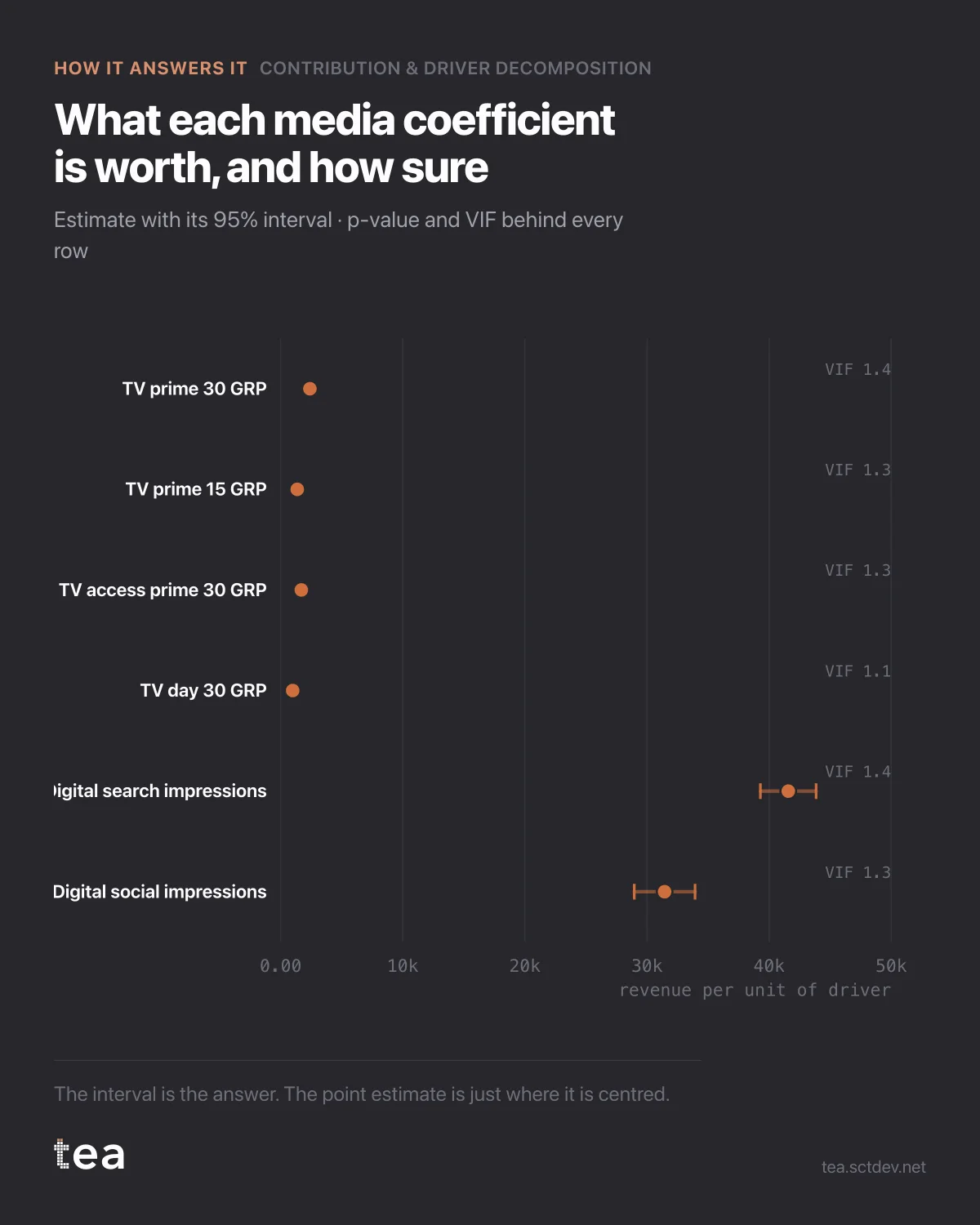
Each row is a media coefficient with its 95% interval: what one more unit of that driver is worth, and how much the data is willing to commit to the number.

The reading is mechanical. An interval that sits well away from zero is a driver you can plan against. An interval that straddles zero is a driver whose effect the data cannot distinguish from nothing, whatever the bar in the contribution chart looked like.

Here every media interval is clear of zero, which is what a clean file with real flight variation looks like. That is the good case, and it is worth knowing what makes it possible rather than assuming it is normal.

Four things behind these intervals:

The standard error. TV prime 30 comes in at 2,396 revenue per GRP with a standard error of 58. That is a tight estimate. Digital search at 41,570 with a standard error of 1,165 is tight too, in proportion. The point estimates are not more trustworthy than their errors.

The p-value, which is reported per coefficient rather than for the model as a whole. A model with an excellent R² can contain drivers that contribute nothing measurable, and the overall fit will never tell you which ones.

The VIF, which is the quiet one. It measures how much each driver's error is inflated by being correlated with the others. The maximum here is 1.9, which is comfortable. Above 5 the coefficients start trading places with each other, and above 10 the individual numbers are not separable even though the total is fine. That is the difference between a model that works and a model whose parts you can quote.

And the residual behaviour. Durbin-Watson at 2.35 on 103 weeks says the leftovers are not strongly autocorrelated, which is the condition under which these intervals mean what they say.

R² is 0.995 and MAPE is 0.52%. Those numbers look wonderful and prove almost nothing on their own: a model can fit history beautifully and still be unable to attribute it. The coefficient table is where attribution is decided.

The habit worth building is small. When someone shows you a contribution chart, ask for this one. If it does not exist, the contribution chart is a set of numbers with unknown error bars, and the size of a bar tells you nothing about whether the driver behind it is real.

It is also the fastest way to spot a model that has been over-specified to look good. Twenty drivers, a beautiful R², and half the intervals crossing zero is not a strong model with some weak parts. It is a model that has fitted the noise and is dividing the credit at random.

The chart is the actual output of Contribution & Driver Decomposition in TEA. The interval, the p-value and the VIF come with every driver.