ea

Analyses/Planning Path/Time Series (ARIMA)

A forecast is only as good as its band.

Time Series fits ARIMA models chosen on your data and forecasts with an interval around the line. The line says where the series is headed. The band says how far to trust it.

Answers What comes next, and how sure can we be? Needs A date and one KPI, 50 periods or more Hands back Model order, AIC, 12-period forecast, 95% band

Twelve weeks of demand, with the band that sets the stock

cases shipped a week, 2026
  • Observed
  • Forecast
  • 95% interval
Interval next week±7%widening to ±15% by week twelve
Weeks the band held94%293 of 312 in a year of backtests
Safety stock1.9 weeksdown from 3, about €450k freed

A frozen-bakery distributor in the Netherlands and Flanders, from the first example below. A composite case: your file picks its own model and draws its own band.

01

What it is for

Most commercial series remember themselves: a good week tends to follow a good week, and the year repeats. ARIMA reads that memory, and turns it into a range rather than a single line with no width.

Sizing stock and staff on a range

A replenishment order or a rota is a bet against the upper edge of demand, not its middle. The band is what the order should be sized to, once it has been shown to hold.

Knowing how far ahead to look

The band widens as the horizon grows. Where it becomes wider than the decision can tolerate, the forecast has stopped informing and started decorating.

Letting the data choose the model

Trend, seasonality and short-range momentum are estimated rather than assumed. The search compares candidate specifications on your file and keeps the one that scores best.

02

How to read it

Five numbers, the forecast with its band, and what the model missed. The block below is the app-installs sample anyone can download, 155 weeks, run with the seasonal option on at 52. Read the numbers in this order, then the residuals.

Weekly installs
Where this is headed -0.8%1 Statistical Method SARIMAX2 Parameters (p,d,q) (1,1,3)3 Model Score (AIC) 817.54 Complexity (BIC) 830.35

Accuracy & Forecast

Residuals Deep-Dive

  1. Where it is headed. The average of the twelve forecast weeks against the last week observed: −0.8%, which the page calls essentially flat. It is the first number on the page, and it is the line only. The band comes with the chart.
  2. The method. ARIMA, or SARIMAX when the seasonal option was on and a seasonal order won the search. Here it did, so the forecast repeats the 52-week cycle it found instead of drawing a straight line through it.
  3. The order. One autoregressive term, one difference to take out the drifting level, three moving-average terms. The seasonal half of the order is chosen in the same search and shows in the shape of the forecast.
  4. The AIC. The score that picked this model among the candidates tried: fit, minus a penalty for every parameter. 817.5 means nothing on its own. It only ranks models fitted to the same series.
  5. The BIC. The same idea with a heavier penalty per parameter, shown beside it for comparison. The search ranks candidates by AIC, and neither number says whether the forecast will hold.

03

Where it sits in the analysis

Time Series is the second step of the Planning Path, after the baseline. Holt-Winters assumes the shape of the series; ARIMA estimates it, and says how far ahead it is still safe to look.

What you carry into the next step is the fitted model and its prediction intervals. Seasonality then names the peaks the model is fitting, and Scenario Simulation bends the plan by the decisions you are considering.

A media effect that lands weeks later looks like autocorrelation to ARIMA. When that is the question, Lag & Carryover measures it directly.

Planning Path

  1. Baseline Forecast

    The trajectory with no intervention in it, which is the only honest baseline for a plan.

  2. Time Series (ARIMA) this page

    Auto-ARIMA picks the specification and argues both sides of the choice, then forecasts with intervals.

    Carries forward: the fitted model and its prediction intervals

  3. Seasonality & Event Impact

    The calendar and the one-off events, so next March is not planned on last March by accident.

  4. Scenario Simulation

    Twenty per cent less media, a price rise, a delayed launch. The plan, under each of them.

04

Where it usually misleads

ARIMA is rarely wrong about its own arithmetic. It is misread at the two ends: what goes in, and how far out the answer is taken.

The line quoted without the band

The forecast line is only the most likely reading of a range. Quoted alone it turns a range into a promise, and the promise is the number that gets repeated in January.

The forecast is always drawn with its 95% interval, shaded around the line.

A horizon longer than the history

Each step forward inherits the error of the step before, and an uncertain slope multiplied by many periods becomes a very uncertain level. Thirty-six months from twenty-six is a fan, not a forecast. Second example below.

tea forecasts twelve periods ahead and no further. A three-year view is a set of assumptions, and belongs in Scenario Simulation, labelled as such.

Residuals that still have a shape

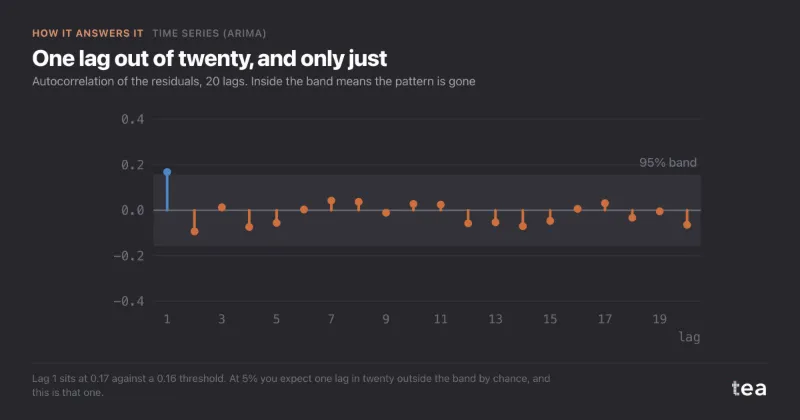
The band is computed as if what the model missed were noise. If the misses run in streaks, or repeat at the same point of the year, the band is narrower than it should be.

Read the residual chart under every forecast before the band: runs of one sign, or a shape that comes back every year, mean the model has left something on the floor.

A model that wins in sample and explodes forward

AIC ranks fit on the history, and says nothing about what a model does when asked to walk forward. A specification with an unstable term can win the comparison and project numbers the series never came near.

The automatic search rejects any candidate whose twelve-period forecast leaves the range of the history, and a model picked by hand that does it is flagged in the notes above the result.

Too short to choose the orders

With little history, comparing candidates mostly rewards the one that follows the noise. The chosen order then describes what already happened rather than how the series behaves.

Scouting a file flags fewer than 50 periods as thin, and the search skips any candidate that has too few observations for the parameters it estimates.

A season seen twice, or not asked for

A yearly term costs parameters that two years of data cannot pay for, and a season that is real but never offered to the model ends up in the residuals.

The diagnostics step looks for a repeating pattern and suggests the seasonal component with its period. The choice stays yours: switched on, the search compares seasonal orders too.

05

Two examples

One file where the band changed a stock rule, one where the band said the question could not be answered. Both are useful results.

Helps

Safety stock sized on the interval

A foodservice distributor of frozen bakery ships about 10,800 cases a week, at a stock cost of about €38 a case. It ordered to last year’s week plus 6%, and kept three weeks of safety stock because nobody trusted the plus 6%.

On 182 weeks auto-ARIMA chose a seasonal model on a 52-week cycle, and the residuals passed: Ljung-Box p of 0.38. The band ran ±7% next week to ±15% by week twelve. Replayed 26 times over the previous year, the model missed by 6.4% twelve weeks ahead, and the band held the actual week 293 times in 312. Sized on the band, safety stock fell to 1.9 weeks: about €450k of working capital.

The backtest that earned the forecast a vote

error twelve weeks ahead, 26 rolling origins

Mean absolute error. The 95% interval held the actual week in 94% of the forecasts, which is what lets you stock to it.
Does not help

Thirty-six months from twenty-six

A pet-food subscription in Spain, launched in August 2024 and now at about 18,400 orders a month, wanted a monthly forecast to September 2029 for a funding round. The file held 26 monthly rows and two Decembers.

Auto-ARIMA rejected the seasonal specifications, and the residuals were clean. The band was the answer: ±12% next month, ±34% by month six, ±75% by month 36, where the central 34,600 orders sat between 8,700 and 60,500. The honest horizon was one quarter. The three-year view became three scenarios, labelled as judgement.

Where the forecast stops being usable

half-width of the 95% band, by month ahead

Two months inside ±20%, 23% by month three, 34% by month six. The horizon belongs on the slide.

06

What the charts add to the numbers

A model order and an AIC tell a statistician what was fitted. The charts tell a planner whether to act on it: how well the past was drawn, what was left over, and how wide the future is.

Accuracy & Forecast

actual, model fit, forecast, 95% band

Reads as: how far does the band open, and does the fit follow the history? On the installs sample the band is about ±6% in the first week and ±12% by week twelve. It is the chart to quote from, with the line and the band in the same sentence.

Residuals Deep-Dive

actual minus predicted, week by week

Reads as: is what the model missed just noise? Not on this file. Two spikes are the model starting up: the first week, which it cannot predict, and the first week of the second year, where the seasonal term begins. Through the second year the misses then swing by several thousand installs from one week to the next. A Ljung-Box test on these residuals, which tea computes with every fit, comes out below 0.001: the band above is narrower than it should be.

Seasonal Pattern: Actual vs Trend

the history against its 52-week average
  • Actual
  • Trend, 52-week moving average

Reads as: how much of the movement is the year and how much is growth. The 52-week average smooths the season away and leaves the level underneath. The distance between the grey and the line, week by week, is what the seasonal term is asked to repeat next year.

tea, the product

Forecast with the band, not just the line

A CSV with a date and one number. The model chosen on your data, a twelve-period forecast with its 95% band, and the residuals that say whether to trust it. Free while in beta, by invitation.

Request a place in the beta

tea, the product

Fifteen econometric analyses on your own CSV: Time Series (ARIMA), saturation curves, elasticities, budget allocation. The diagnostics shown, and a plain sentence when the file cannot answer.

Free while in beta, by invitation.

Request a place in the beta →

Now run it on your own data.

tea runs Time Series (ARIMA) and fourteen other analyses on any weekly CSV, in minutes. Free while in beta, by invitation.

Join the beta